PiFi SLAM
A Spring 2020 ECE 5725 Project
By William Laney (wel53) and Luke Puchalla (lcp77)
Demonstration Video
Objective
Our goal was to solve the simultaneous localization and mapping (SLAM) problem by using WiFi measurements. Specifically we wanted to implement this paper, where they solved SLAM through a Graph SLAM formulation with WiFi signal strength and movement data from an IMU. Due to the constraints of graph SLAM, data would first be collected, and then SLAM would be computed offline
Introduction
This project was executed remotely, meaning all design and testing was done separately or collaboratively over zoom. The only soldering required was for the IMU, which was also the only additional part we had to order. System assembly was quite simple; the actual work was in writing the code. First, we developed methods of collecting data from both the WiFi receiver and the IMU. Next, we wrote the actual SLAM algorithm, as well as a script to perform dead-reckoning, meaning to resolve a path of where we think the device travelled solely based on IMU measurements. A large amount of time was spent study the math needed to implement the SLAM algorithm. After writing the SLAM code, we developed unit tests to confirm our code’s functionality and accuracy. We also wrote a script that consolidated the IMU data such that, in the SLAM algorithm’s perspective, the same number of WiFi measurements were taken as IMU measurements. Finally, after creating a script to display both the WiFi SLAM plot and the dead reckoning plot, we wrote a control script to launch all of the previous scripts mentioned in the appropriate order, completing an end-to-end working embedded system.
SLAM Overview
SLAM stands for Simultaneous Localization and Mapping, meaning the device can map the environment it is in and localize (determine where it is on the map at the given moment). In this project, we implement Graph SLAM, which is one of many methods of solving SLAM. The basic idea of SLAM is that a robot’s movement sensors are imperfect, and using a separate set of measurements about landmarks in the environment (in this case, signal strengths from nearby wireless access points) can help resolve the probability of certain movement measurements. This is done by formulating equations called measurement functions that take in a belief about the world, and output what the sensors would read if that belief was true. These guesses of the sensor measurements are then compared to the true measurements, and the difference between them is used to correct the belief about the world.
WiFi SLAM
The idea of WiFi SLAM is to solve the SLAM problem by passively using the WiFi signals available in most modern indoor built environments. In order to do this, we choose to implement the research paper “Efficient, Generalized Indoor WiFi GraphSLAM”. This paper was an appealing choice for a number of reasons. First, is that algorithms can work in sparse WiFi environments, meaning not many wireless access points are needed to get results. The second is that it used a simple sensor setup, just an IMU and standard WiFi receiver. Finally, the real world experimental results published in the paper were impressive, but still seemed achievable.
For the purpose of this report, “Efficient, Generalized Indoor WiFi GraphSLAM” can be thought of as having two parts: creating a WiFi prediction model, and formulating the WiFi SLAM problem so that it can be solved with Graph SLAM. The main things to know about Graph SLAM for this report are that it is an offline SLAM solver, meaning all the data is collected before SLAM is solved, and that it can be set up as a non-linear least squares problem. For more information about Graph SLAM, and alternative SLAM techniques, please see the References section.
The SLAM algorithm in the paper takes in three inputs:
- Angular velocity from gyroscope
- Distance from a “pedometer”
- WiFi signal strength measurements
They formulate their state space, their representation of the world, in terms of three parameters:
- Distance traveled per time step
- Angle that distance was traveled in
- WiFi signal strength
The output from the algorithm is the best estimate of this state space.
The distance traveled per time step and angle traveled can converted to the robots X-Y position through the following function:
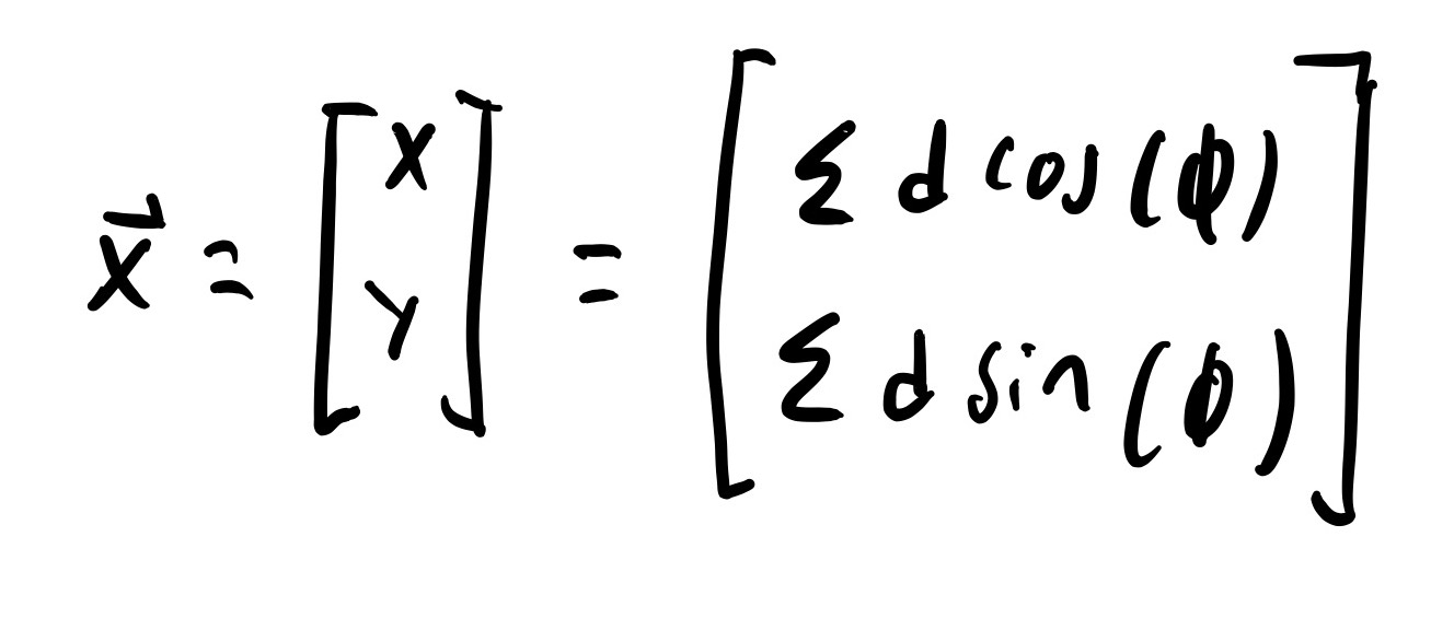
State Space Conversion
The authors chose to use distance traveled and angle instead of more traditional X-Y coordinates because it makes the math easier at some points in the algorithm.1
WiFi Measurement Function
Coming up with a way to predict WiFi measurements based in part on location is the most important step in the paper. This sort of measurement model is needed for all traditional SLAM solving techniques, and is difficult to formulate for RF signals like WiFi.2 The problem with determining a measurement model for WiFi signal strength is that WiFi signal strength is highly dependent on building geometry and materials. If the robot knew enough about the environment to fully predict WiFi signal strength, it would already have a highly accurate and detailed map, and thus not be solving SLAM. To get around this problem, the authors of the paper do not try to perfectly predict the WiFi signal strength, they just try to make a good enough prediction and use it to compensate for the error in the IMU measurements.
To predict a single WiFi measurement, the authors take a weighted mean of all the other WiFi measurements from the same wireless access points. Formally, this is:
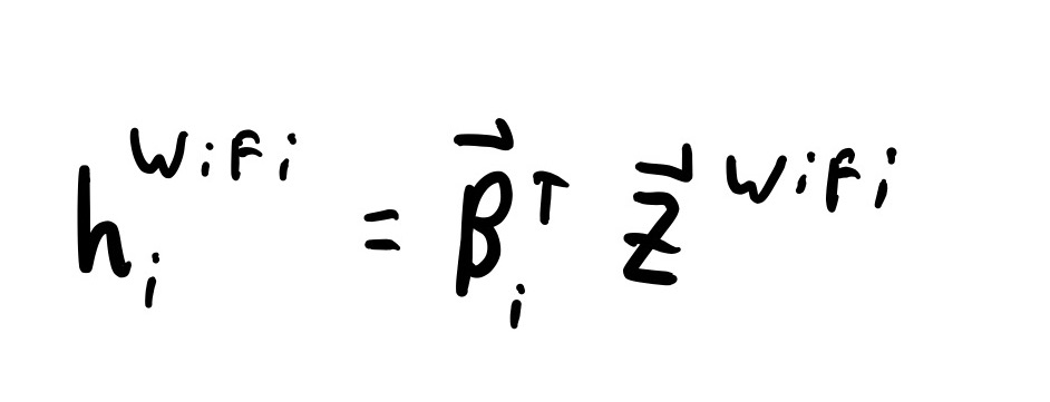
WiFi Measurment Function
Where Β is the weights, and Z is the WiFi measurements from the access point. The value of Β for the WiFi measurement being predicted needs to be set to 0. This is to insure that the real measurement at point i is not being used to predict the measurement at point i.
The weights for this weighted mean are generated using the following function:

Weight Function
This function is a gaussian kernel and essentially gives the probability that two WiFi measurements are near each other and only separated by free space. Xi and Xj are the believed XY positions of the two WiFi measurements, and Tau is a constant representing the average distance between walls. The paper used 2 meters for this but shows that the value does not matter too much within reason.
There are three important things to note about these weights. The first is that they are based on euclidean distance between WiFi measurements. This means that you must convert out of the Distance-Angle position representation to and X-Y position representation to calculate the weights.
The second is that these weights can not be used to directly make the Beta vector. Before multiplying the Beta vector by the WiFi measurements vector, Beta needs to be normalized so that it sums to one. This makes the weights valid for the weighted mean.
The the third is since we are averaging WiFi signal strengths, the signal strengths themselves must be in units of mW or Watts, not dBm.
The question of whether this WiFi measurement function is valid for use in SLAM will mostly be left as an exercise to the reader. In general, this sort of gaussian kernel for signal strength prediction is supported by the literature. We additionally present some basic and non-rigorous tests of it in our Testing section. We do believe that this measurement function technique is interesting, and worth further research, but are still not 100% convinced of its efficacy.
Solving Graph SLAM
The most important point in understanding the author's graph SLAM solution is understanding how they represent their state space. Remember, the state space is the robot's beliefs about the world. Traditionally, the state space is represented as a matrix with each row corresponding to a time step where measurements were taken, and each column to a different state space variable. An example can be seen below:
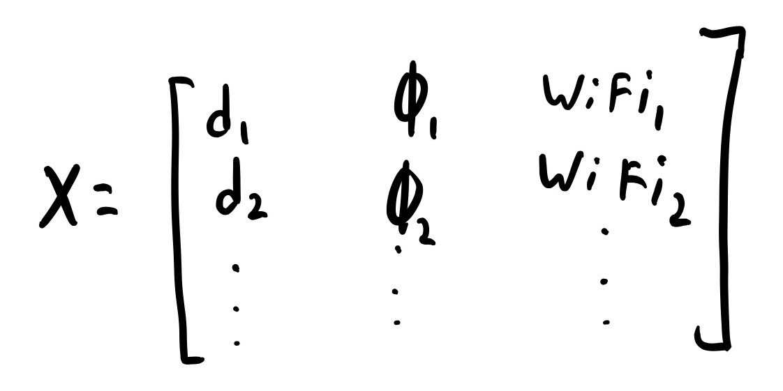
Tradional State Space Matrix
In this matrix each row corresponds to a time step where distance, gyroscope, and WiFi measurements were taken: the first column is the believed distance at this time step, the second is the believed angle, and the rest are the believed WiFi signal strengths.
This is not how the authors chose to represent their state space. To the best of our understanding, they formulated their state space as a single column vector. The first set of rows in the column are the distance measurements, the second are the angles, and the remaining rows are the WiFi measurements. This is essentially taking the matrix shown above, cutting the columns out, and stacking them on top of each other as shown below:
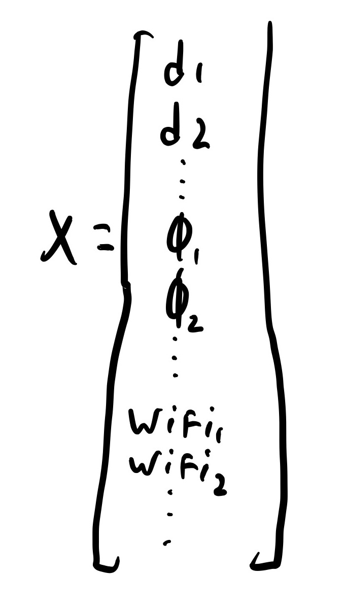
State Space Matrix Used
Once the state space is formulated in this way, the authors proceed to solve Graph SLAM through the Gauss-Newton algorithm, which is a technique for solving non-linear least squares problems. The formulation for this problem can be seen below:
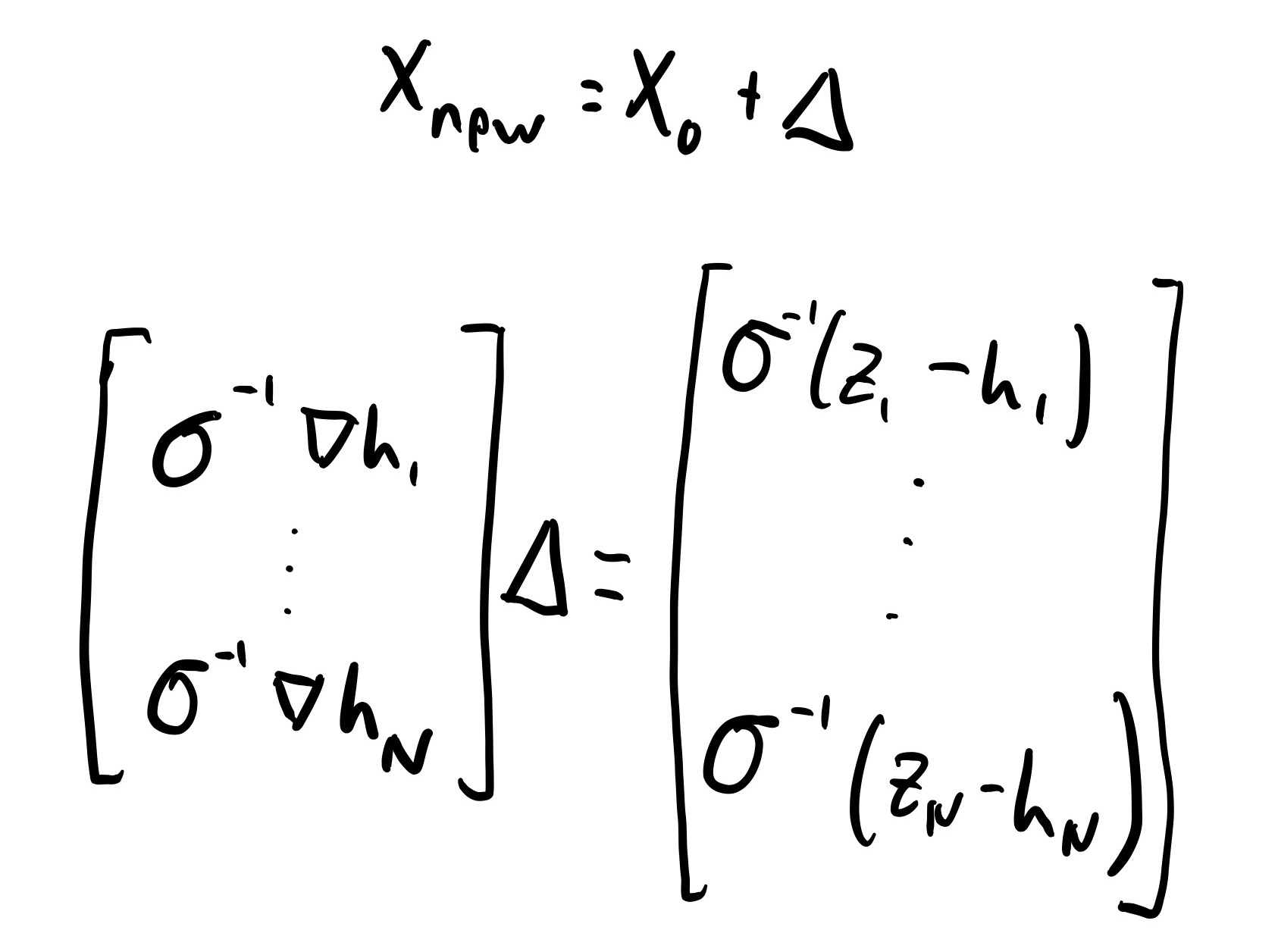
Guass-Newton Formulation
Here, X0 is the initial state space estimate and Δ is a correction to it. Δ is found through solving the shown matrix system. The matrix on the far left is the Jacobian of the predicted measurement functions with respect to the state space. The way it is represented above shows that each row in the Jacobian is the derivative of the proper measurement function with respect to all the state space variables. The vector on the far right is the difference between the true measurements and the predicted measurements from the current state space belief.
The calculation of the predicted WiFi measurements was covered in exhausting detail above. Calculating predicted distance measurements is trivial because the state space is already defined in terms of distance. This means that state space distance can simply be subtracted from the measured distance. Calculating predicted gyroscope measures is straightforward and can be seen below:

Gyroscope Measurment Function
This prediction technique implicitly assumes that all the angles have equal time steps between them, but this is a good assumption.
The inverse sigmas seen on each side of the equation correspond to the inverse standard deviation of the sensor measurement noise.
Before explaining how to take the measurement function derivatives to create the Jacobian matrix, a note on dimensionality of this equation. Δ must be the same size as the state space so that it can be added to it. The vector of differences between expected and true measurements on the right side must be equal to the number of measurements. Due to the definition of the gyroscope measurement prediction function, there must be one more angle in the state space than gyroscope measurements. To keep things balanced, there also must be one more distance in the state space than distance measurements (we put this extra distance at the end and set it to zero). This means that the Jacobian matrix on the far left is not square; it has a number of rows equal to the number of measurements, and a number of columns equal to the number of state space values. This is necessary for the matrix multiplication to be possible.
To get the derivatives for the Jacobian function, we need the general derivative for the three types of measurement prediction function. Which general derivative is used in which row of the Jacobian is determined by which measurement function was used in the corresponding row of the real minus prediction vector. Each row of the Jacobian matrix is different, because each corresponds to a different measurement, so different values are plugged into the corresponding general derivative function.
The derivative of the distance prediction function with respect to the state variables is easy. It is a row vector where all the elements are zero, except for the one corresponding to the distance state being compared to the distance measure. This element is 1.
The derivative of the angular velocity function is similarly straightforward. The row vector is all zeros except for two elements. The one corresponding to the i angle is -1 and the one corresponding to the i+1 angle is +1.
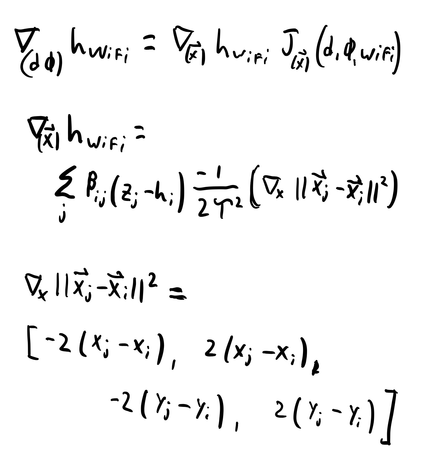
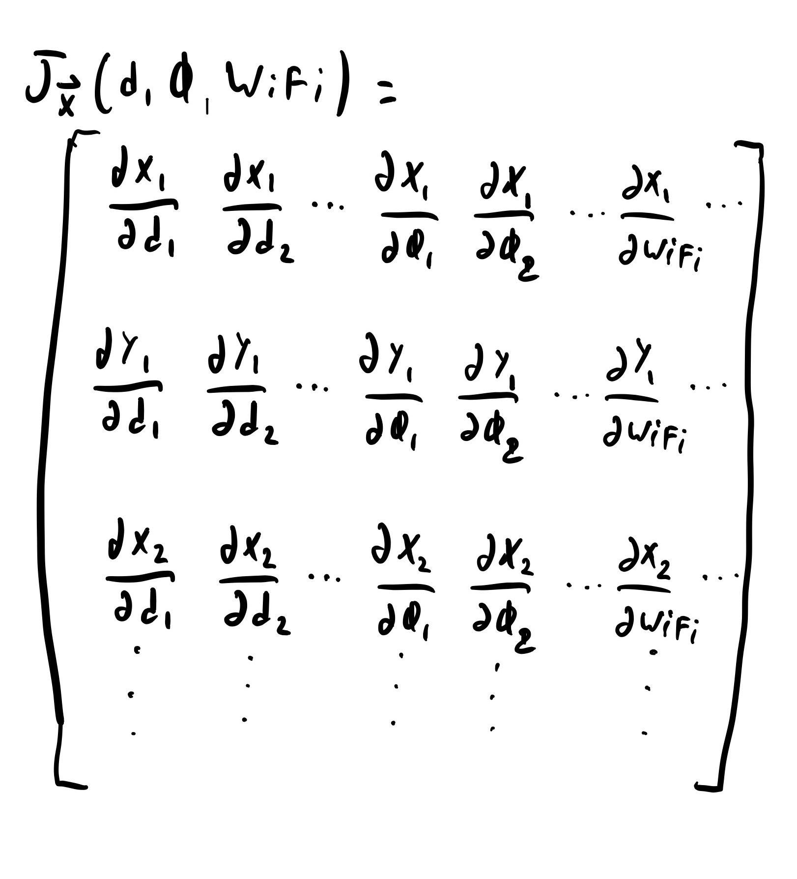
The derivative of the WiFi prediction function is messy. As noted in the WiFi prediction section, the WiFi prediction must be solved with the state space in terms of X-Y positions for the euclidean distance, but the state space is represented and stored in terms of distances and angles. This means that to take the derivative of the WiFi prediction function with respect to the distance and angle state space, the Jacobian of the distance angle state positions must be found and multiplied by the derivative of the WiFi prediction function taken with respect to the X-Y positions.
The necessary derivatives and Jacobians are shown below. The result is a row vecotr with a number of collums each to the number of state space variabels. Note that the distance-angle state space Jacobian includes a large number of derivatives taken with respect to WiFi measures. All of these derivatives are zero.
WiFi Measurment Function Derivative
After solving for Δ and correcting the state space estimate, this whole matrix system is solved again using the new state space estimate. This process repeats until the state space estimate converges, where convergence is the change to the state space on each iteration passes below a threshold.
When the state space does converge, the final set of distance and angles is the path of the robot.
Design
Overview
Observe the block diagram below:

System Block Diagram
As described in the introduction, each of these blocks represents a different script in the codebase. The user pushes button 17 on the piTFT to start both data collection scripts in parallel. The WiFi data collection script and the IMU data collection script must run in parallel because we want to take data data from the WiFi sensor as quickly as possible, while mantaining a constant sample rate with the IMU. Once the user is done collecting, they hit button 17 on the piTFT again, and the rest of the work is up to the software. The datasets output from both of the scripts is then taken as an input to the data association script, where IMU data is consolidated to match the number of WiFi measurements. These datasets are then used by the WiFi SLAM script to solve SLAM as described above. After performing dead reckoning, both the dead reckoning plot and the WiFi SLAM plot are displayed on the piTFT, where the two middle buttons may be used to scroll through the list of plots.
A schematic for the IMU electrical connections can be seen below:
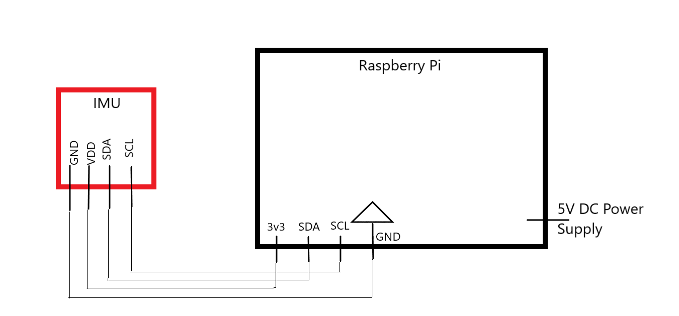
System Electrical Schematic
IMU Data Collection
Bring up and Initial Testing
We chose to use the LSM9DS1 inertial measurement unit (IMU) mounted on a breakout board from sparkfun for this project. The LSM9DS1 is a nine degrees of freedom (DoF) sensor, meaning it has three axes of accelerometer, gyroscope, and magnetometer data.
We only ended up using 2 DoF in this project: one accelerometer, and one gyroscope. But, we wanted to get a 9 DoF sensor because we were unsure of how we were going to implement the SLAM algorithm when we made our sensor selection.
We chose this IMU for the following reasons:
- It is well supported in the community giving us a variety of libraries and sample code.
- It is a 3.3V device so it can interface directly with the Raspberry Pi GPIO pins.
- The magnetometer has better sensitivity than other similar 9 DoF sensors with a least significant bit of 0.14mGauss. The gyroscope and accelerometer were about the same as most other devices in this price range. This extra sensitivity did not end up mattering because we did not make use of the magnetometer in this project.
- The sensor supports both I2C and SPI communication, giving us extra flexibility in the hardware setup.
We interfaced with the sensor using I2C and the Adafruit LSM9DS1 circuit python library. Circuit python is a python implementation developed by Adafruit to run Python on microcontrollers. Adafruit additionally released libraries to allow Circuit Python to run within CPython in non-microcontroller environments. We were initially hesitant to use a library that was designed to run on a microcontroller and ported back to normal Python, but it worked without any issues.
We conducted initial characterization of the sensor where we tested how fast we could sample from it using the Adafruit library, and found the variance of the measurements when it was not moving.
To test sampling speed, we took a set number of samples in a loop and timed the loop completion. We found that we could sample accelerometer and gyroscope data at about 400Hz, and data from the accelerometer, gyroscope, and magnetometer at about 285Hz. The reason for the speed decrease when including the magnetometer is that the magnetometer data is stored in a different set of registers and requires connecting to the IMU at a different I2C address to access. These sampling speeds are more than sufficient for this project.
To test variance, we let the device lay motionless on a table for 10 minutes while collecting data. We found a variance of roughly 0.00016 m/s2 on the accelerometer axis, and 0.021 deg/sec on the gyroscope.
For more discussion of IMU testing, please see the Dead Reckoning section.3
Description of Final Code
For data collection to feed into WiFi Slam, we sampled the gyroscope and accelerometer at 20Hz, and wrote the output to a CSV file. We did this by first opening a CSV file buffer and then entering a sampling loop where we sampled the sensor, took a time stamp, wrote the data as a new row to the CSV, and then entered a 0.05s sleep. While this does not give exactly 20Hz sampling due to the execution time of the code, and the non deterministic behavior of both Python and Linux, it was close enough for us to get good results.
Before entering the main data collection loop, we print a message to the screen instructing the user not to move. We then collect 10 samples and print a second message telling the user to move. These 10 samples are used to calculate offsets in the accelerometer data due to gravity/normal force. Again please see the Dead Reckoning section for more details.
Finally, the script made use of two buttons built into the PiTFT. The first was button 17 that indicated the user would like to begin sampling data or the user would like to stop sampling data. The second was button 27, which was an emergency exit that quit the program immediately. Both of these buttons were set up as hardware interrupts that would trigger on a falling edge. We had to add a debounce time of 400ms to pin 17 to prevent situations where the device would start taking data and immediately stop because of transients from the button press.
WiFi Data Collection
For WiFi data collection, we used the onboard WiFi receiver. This is to maintain consistency between testing on our two separate Pi’s, since the onboard WiFi adapters are assumed to have more similar variance than WiFi dongles from different manufacturers. However, a much better WiFi dongle can easily be used in this project.
We use the following command to poll the onboard WiFi receiver: sudo iwlist wlan0 scan
This command gathers lots of information about all of the access points seen by the onboard receiver. Below is an example of the command’s output for a single access point:
Cell 01 - 	Address: 28:80:88:F2:98:AA
	Channel:1
	Frequency:2.412 GHz (Channel 1)
	Quality=45/70  Signal level=-65 dBm
	Encryption key:on
	ESSID:”Router I hardly know her-2G_EXT”
	Bit Rates:1 Mb/s; 2 Mb/s; 5.5 Mb/s; 11 Mb/s; 9 Mb/s
		    18 Mb/s; 36 Mb/s; 54 Mb/s
	Bit Rates: 6 Mb/s; 12 Mb/s; 24 Mb/s; 48 Mb/s
	Mode:Master
	Extra:tsf=000000000000000
	Extra: Last beacon: 80ms ago
We are only interested in two things: identifying distinct access points across collection samples, and determining their corresponding signal strength. Thus, to filter out useless information, we pipe this command into an egrep as follows: sudo iwlist wlan0 scan | egrep “Cell|Signal”
Each “Cell” line is a different access point reading, so we must collect information about each “Cell” in the output. This line also contains the access point’s MAC address, which is critical to uniquely identifying all access points that we see. We use the access point's MAC address instead of the SSID (network name) of the network because multiple access points can broadcast the same SSID. The line containing “Signal” contains the signal strength in dBm from that access point. The above command yields access point information in the following condensed format:
Cell 01 - 	Address: 28:80:88:F2:98:AA
		Quality=45/70  Signal level=-65 dBm
Cell 02 - 	Address: A8:9A:92:A1:9B:89
		Quality=61/70  Signal level=-42 dBm
...
This format can be easily parsed with regular expressions to determine the MAC address and signal strength of each access point from each collection.
The method of collection is simple. We create a 2D list, where the first element of each entry is the timestamp of collection, and the second is the actual string output from the command.
After collection is finished, we loop through the entire list and extract the useful information with regular expressions. The targeted information is highlighted below:
Cell 01 - 	Address: 28:80:88:F2:98:AA
		Quality=45/70  Signal level=-65 dBm
By the end of the script, a CSV file is created, where the first column is a timestamp, and the remaining columns correspond to readings from specific access points. Each row represents all of the signal strengths taken in that timestamp. This means that each column after the time column represents all of the readings from a single access point; if a signal was not received by a specific access point anytime during collection (after the access point was “seen” earlier), we fill the space with a Not-A-Number.
The script functions with the same GPIO setup as the IMU code, so that when they are launched in parallel in the control script, when button 17 is pressed, both the WiFi script and the IMU script start collecting. This is explained in more detial in the Integration section.
WiFi Data Collection Testing
One major issue we first encountered when using this command was how frequently we would be able to poll the adapter for information. We found that polling as fast as possible would throw an error saying the receiver was “busy” or “didn’t support scanning.” We found that the amount of time spent each loop iteration updating the data collection list mentioned earlier was normally sufficient time to delay each command execution. We found that we could collect WiFi data at a max of around 0.75 - 1 Hz. We also implemented a try/except block such that the code would not immediately quit if the receiver threw an error. Instead, the program would simply move on and continue collecting measurements.
Data Association
After both IMU and WiFi data are collected, we must format the data into matrices that the SLAM algorithm will accept. Two steps are taken to format the data. First, we consolidate the IMU data such that there is only one set of IMU measurements per set of WiFi measurements. This is due to the way the SLAM algorithm is implemented. IMU data can be collected at roughly 20 Hz, whereas the WiFi data is collected only at about 1 Hz. For every WiFi measurement time, we sum all of the distances recorded by the IMU since the last WiFi collection, and we average all of the angular velocities recorded since the last WiFi collection.
Second, we scrap the timestamps for all of the data. This is done after the first step because the time stamps are nessary in that step.
WiFi SLAM Implementation
We chose to implement WiFi SLAM in a way as similar to the math formulation as possible. This was done to make it easier to write the initial code and to validate what was put forward in the paper. Writing the code in a highly analogous way to the math was not good for computational performance, as the easiest way for a human to solve a math problem is rarely the easiest way for a computer to solve it. For example we re-arranged and transposed matrices multiple times in a way that helps when solving by hand, but is not strictly necessary to do. Our plan was to get the algorithm working with poor performance, validate it, and then work on performance improvements.
We did not get the chance to make these performance improvements, or even rigorously profile the code and determine which funcions were causing bottle necks. For datasets that were around a minute in length the SLAM algorithm converged in a matter of seconds. When we tested a ten minute data set, the algorithm took over ninety minutes to converge. We believe that this poor performance can largely be attributed to the size of the matrices associated with larger datasets. Keeping all the matrices in memory at once may not be possible on the Raspberry Pi, leading to large amounts of time spent swapping. Additionally there are multiple calculations in the algorithm, such as calculating the Jacobian matrix, that could be performed in parallel, but were not.
From a software architecture perspective, we implemented the algorithm within a class. The class had a main function that generated the matrices for the matrix equation that needed to be solved, solved the equation, and updated the state vector. It generated the matrices by calling into other class functions that performed the various steps in the algorithm, such as generating the weight vector, generating WiFi predictions, or assembling the jacobian matrix.
As far as the implementation, we made heavy use of NumPy. NumPy is essentially the standard for mathematical computing in Python. One of it's benifits is that is has many useful functions relating to linear algebra. In order to solve the matrix algebra problem presented in the WiFi SLAM section, we used the NumPy linear algebra least square solver. This worked well in that it always gives results regardless of the data in the matrices given, however it may not have been the most appropriate choice for this problem. Outside of performance improvements, an area of future work for this algorithm would be to investigate linear algebra matrix solvers more closely.
Finally, the algorithm was given a maximum of five iterations to converge. It never hit this limit without converging on a solution. The convergence criteria was set as all the state space variables changed by less than 0.1. This was an arbitrary criteria and deserves more research.
Dead Reckoning
Dead reckoning is the process of estimating location based only on movement data. For this project, we need dead reckoning techniques for two reasons. The first is to get the distance we traveled in each time step, which is an input to WiFi SLAM. The second is to generate trajectories we can compare to the outputs of WiFi SLAM. The distances are from the IMU accelerometer data. The full trajectories are from combining the accelerometer data with the gyroscope data.
Acceleration is the second time derivative of displacement. This means to get distance measures from an accelerometer, we must integrate twice with respect to time. This yields the basic kinematics equation shown below.

Linear Kinematics Equation
V is the velocity and X0 is the initial displacement. Velocity comes from integrating accelerometer data once and adding the initial velocity. We solve the above equation for each acceleration measurement. In the first iteration, we take the initial displacement and initial velocity to be zero. In every subsequent iteration, we take the initial displacement and velocity to be the value found in the previous iteration.
Getting angles from gyroscope data is a similar process. Gyroscopes give angular velocity, which is the first time derivative of angle. To retrieve the angle, we simply integrate the gyroscope data once with respect to time. The resulting equation can be seen below. Again we take the first initial angle to be zero.

Angular Kinematics Equation
While the above dead reckoning formulation is simple and based on 101 physics, it does not yield good results in the real world. This is because of error in the sensor. The error accumulates through these integrations over time and is never corrected for. This causes the dead reckoning trajectory to diverge from the true trajectory. More advanced approaches to dead reckoning, such as the use of Kalman filters, can be used to improve results.
In our implementation, we solved dead reckoning with the naive approach shown above. Furthermore, we only used one axis of accelerometer data, and one axis of gyroscope data for our results. This simplified the math at the expense of accuracy.
We took several steps to improve the accuracy of our results. First, we applied a moving average filter to our acceleration data. For each acceleration measurement, we averaged it with the three measurements before and the three measurements after. This smoothed out the input data, which could be quite noisy, as seen below:
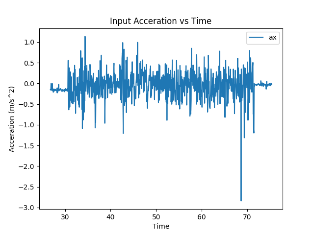
Raw Acceration Data
Second we averaged the first ten acceleration measurements and subtracted this value from all the other measurements. This was done to correct for any normal force acceleration we may have seen.4 This subtraction generally worked well, but if the angle of the IMU shifted, the magnitude of the normal force on each axis would change, removing the effects of this subtraction.
Dead Reckoning Testing
To test and validate our dead reckoning results, we generated a number of statistics and plots. These statistics and plots first helped confirm that the data taken from the IMU data collection code was valid. They also confirmed that the dead reckoning was performing as expected. A set of statistics can be seen below:
Number of data reads: 658
Time accounted for: 35.245476288000006
Max time between readings: 0.06054765599999712
Average time between readings: 0.053726282480974136
Meadian time between readings: 0.05368802099999925
These show that the sampling frequency and timing information of the data set is correct. They also give information about the number of samples.
We then plotted the raw accelerometer and gyroscope measurements. This helped us insure that the sensors were giving sensibel information. Example plots are shown below:
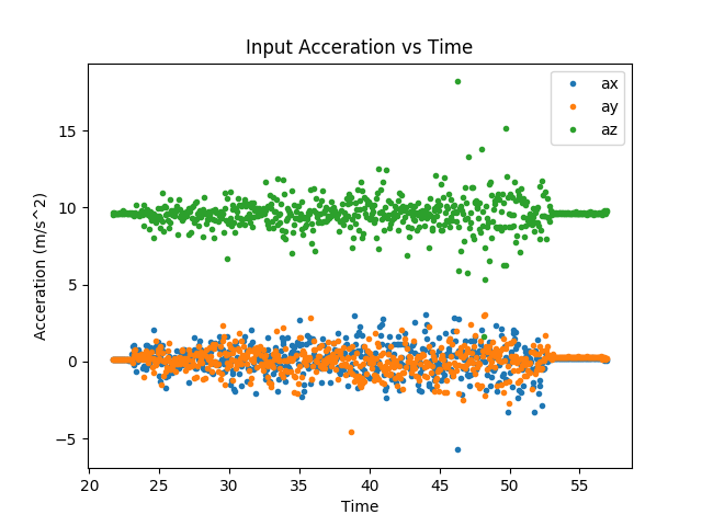
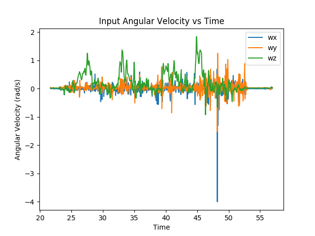
Raw accerometer and gyroscope data
Finally, we made plots of the systems velocity, displacment, and trajectory (X-Y positions of the system in space, assuming the initial measurement is the origin). We compared these results to baselines we took by moving the system around and measuring the distance we moved with a tape measure. Example plots are shown below, all plots in this section were generated with the matplotlib Python library.
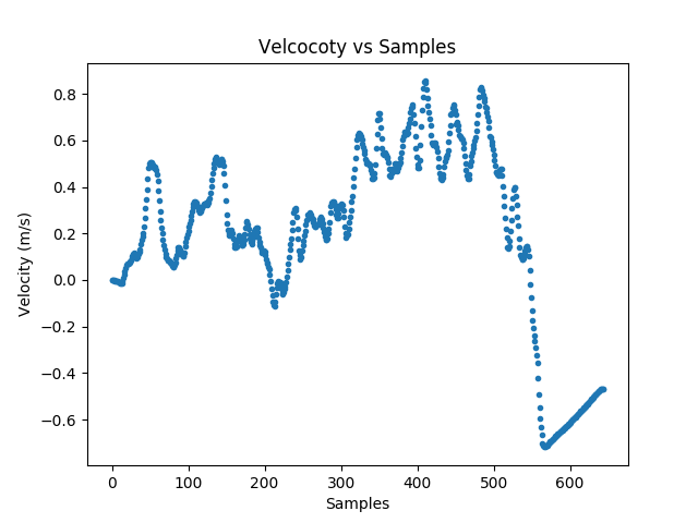
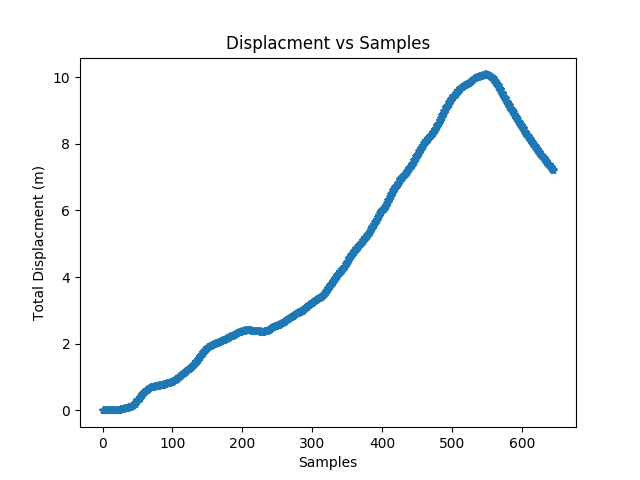
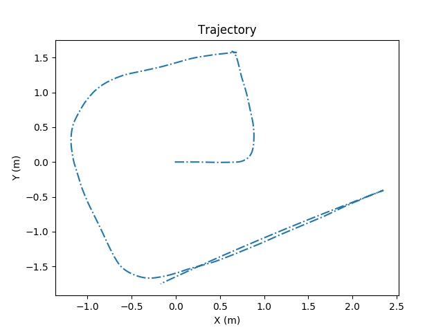
Example Velocity, Displacment, and Trajctory Plots
We subsequently realized we could not carry the system in our hands to get good results. We could not hold the system level enough for our normal force correction to work. Additionally, the acceleration seen by a foot fall while walking could be seen in all three axes, and our filtering could not compensate for that. Because of this, we took all data sets by either dragging the system around (as seen in the video) or by putting it on something with wheels.
The Mystery of the Missing Time
At one point, while testing the dead reckoning, we noticed that we would get drastically incorrect results. After investigating, we discovered that sometimes our timestamps would jump many seconds. Below is a plot of time plotted against itself from one of these jumps.
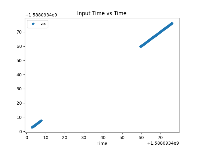
Time assosated with the ax axis plotted against itself
Since the code was set up to sample at 20Hz, these jumps were unexpected. Since the dead reckoning relies on time, it would set a constant acceleration for the duration of the time jump and greatly alter our results. We determined that the cause of these jumps was how we were getting times for our timestamps. We were using the python function time.time(), which returns the UNIX time. However immediately after booting the Raspberry Pi this time would be incorrect and then jump to the correct time when the Pi connected to the internet and could contact a time server.
To solve this problem, we switched from using time.time() to using time.clock_gettime(time.CLOCK_MONOTONIC_RAW). What this new function does is return the time in seconds since the system booted. This is not subject to corrections from the time server. We are able to use it because the only metric that is important to our analysis is the time between samples, not the wall clock time.
TFT Plotting
In this script, we use the pygame library along with GPIO to enable the dead reckoning and SLAM plots to be viewed and toggled between on the TFT screen. The plots are output from the dead reckoning code and the SLAM code as png files. We used the techniques we practiced in lab sessions "blit", in pygame parlence, these png files to the screen. Rather, Would begin by displaying one of these plots (the SLAM plot). The user would be able to toggle between this plot and the dead reckoning plot by using buttons 22 and 23 on the TFT. The plots may be scrolled through as a wrap-around list. The wrap around list formuation was used to make it easy to add more plots in the future, if we choose to do so.
TFT Testing
The only issue we had with displaying plots on the TFT was that sometimes they would be different sizes, so on different runs of the program, the screens would have varying sizes of black margin on the borders of the screen. The size diffrences in the plots was caused by matplotlib. In that library plot sizes are spefied in units of inches, but this does not garuntie the same pixel size plot ouputs. We fixed this in pygames by 1) centering each plot and 2) making the background white. This makes the display look much cleaner.
Integration
We launch all of the scripts above in a single control script. We utilize the multiprocessing library to run the two data collection scripts in parallel, using a pool of workers. In this control script, we also pass filenames and file paths to different scripts when we call them for execution. We first create a directory name that the data will be written to at the beginning of the file. We pass this directory name to the data collection scripts. The scripts then write their respective data CSV files to this directory. Next we pass the file paths of the data files to the data association script. The data association script returns two matrices: measurement data and WiFi data. These matrices can be passed inside the control script to the WiFi SLAM script. The WiFi SLAM script and dead reckoning script both output their png plots to the same directory used throughout the run. These plot file paths are finally passed to the TFT script.
Integration Testing
We had some troubles with using the right file paths and passing them correctly to different scripts. This was worked out rather quickly though through trial and error.
The only other problem we had was that the buttons for scrolling through TFT plots were not working when the TFT script was integrated into the control script. This was because in the TFT script all of the GPIO setup was being done outside of the class. Thus, the GPIO setup was being executed upon import of the TFT file into the control script. This meant all of the TFT GPIO was being cleaned up once the data collection scripts called GPIO.cleanup(). To solve this, we simply moved all of the GPIO setup into the TFT class init method.
Testing
Unit Testing
To give ourselves confidence that the WiFi SLAM functioned as expected we wrote several unit tests using the unittest Python library. These are mostly small problems that could be worked out by hand. We used these tests to confirm matrix dimensions in the slam solver; if the matrix dimensions didn’t match what we expected, we’d know there was a problem. The tests were also used for accuracy. Several tests ensure that NaNs in the WiFi data are handled correctly. Additionally, we have one test with actual numbers to see if the functions work correctly with some arbitrary data.
Implementing this unit testing did revealve bugs in our original WiFi SLAM code. These bugs became obvious with the unit tests and were quickly corrected.
End-to-End Testing
Full system end-to-end testing was somewhat limited by COVID-19 quarantine restrictions. The only areas available for us to test the performance of the WiFi SLAM algorithm were William’s parents’ house, and Luke’s collegetown house. For the remainder of this section, we are going to focus on tests and results from William’s parents’ house. William set up a test area in his basement by laying out a series of tape measures. He then moved along the tape measures compared the algorithm results to the path he travled. An image of this setup can be seen below
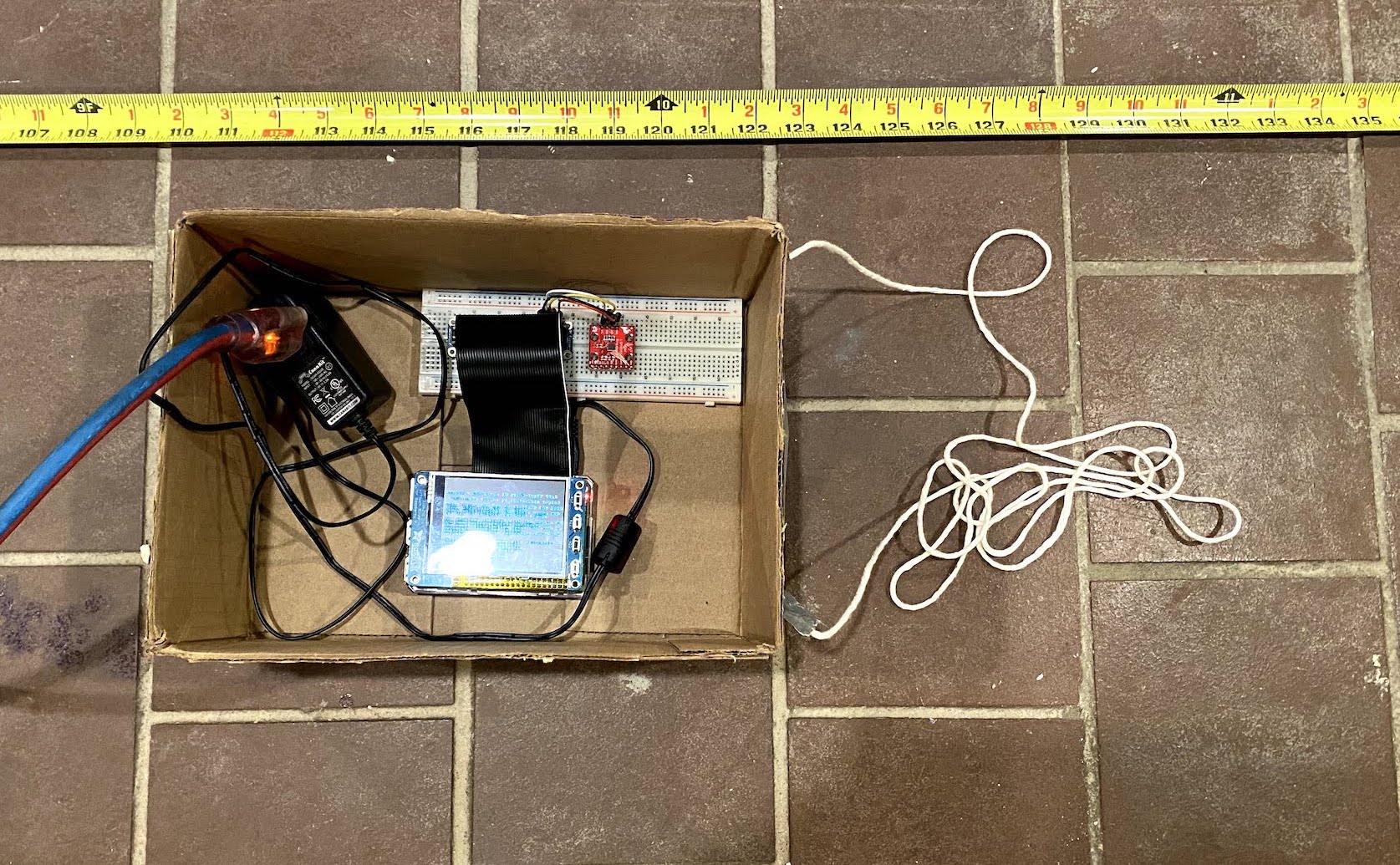
Tape measure and box test setup
We found that both the dead reckoning and WiFi SLAM results generally had large error. We found that when moving in a straight line the WiFi SLAM was able to provide better results than the dead reckoning. An example of this is shown below. For this experiment, William moved 2 meters in a straight line along the positive X axis. Both the dead reckoning and slam got the X distance approximately correct, but the dead reckoning showed a half meter of movement in the Y direction that did not happen. WiFi SLAM, on the other hand, only showed about 20cm of movement in that axis.
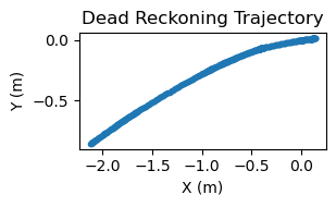
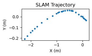
Trajctories from moving 2m in a straight line
These improvements were not seen in test cases that involved turning. The next two plots show the results from moving in a 2-meter by 2-meter square. The dead reckoning did a poor distance estimation in this case, but it did get a rough idea of the movement shape. The WiFi SLAM did not. This is probably due to the gyroscope averaging done in the data association step.
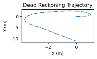
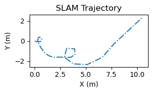
Trajctories from moving in a 2m square
Finally we found that the accelerometer was highly sensitive to the bad normal force removal. The following plots show a case where the accelerometer tilted slightly after we began moving, this led it to constant acceleration that was not filtered out. This constant acceleration led to increasing velocity and thus rapidly increasing displacement.
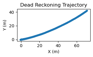
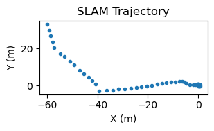
Trajctories without the normal force fully removed
WiFi Measurement Function Testing
The WiFi measurement function is the key component to our WiFi SLAM implementation, and, we believe, the key innovation of the paper we are trying to implement. Most of the analysis and use of this function comes from our use of it within the larger WiFi SLAM algorithm, but we did conduct a basic test to see if it worked in isolation. We placed our Pi setup 1 meter from a UniFI Dream Machine wireless access point. This device has a max rated Tx power of 23dBm in the 2.4GHz band. At 1m we read a signal strength of -30dBm on the Pi. We then moved the Pi 2m from the Dream Machine and read a signal strength of -39dBm. At 3m, it read -37dBm. This already shows the issue with RF signal strength: we moved farther from the access point but the signal got stronger. A picutre of the test setup used to get this data is shown below:
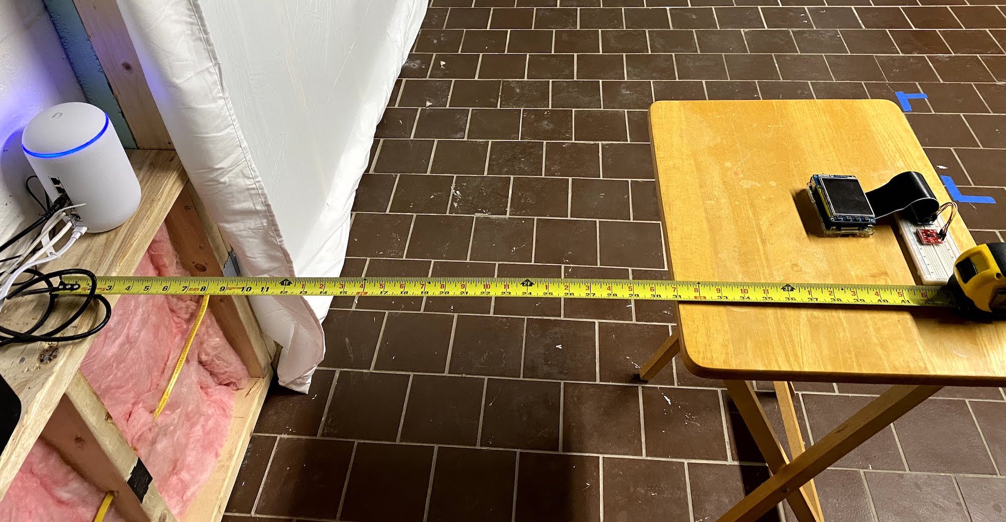
Raspberry Pi 1m from a wireless access point
We can use the 1-meter and 3-meter measurement to predict the 2-meter measurement by a simple average. The weight function gives the non-normalized weight for moving one meter as 0.78, but since we only have two equal distances, this normalized to them being weighted equally. This makes a predicted measure of -32dBm (remember to do your averaging in mW), when the true measure is -39dBm.
Similarly, using the 2-meter and 3-meter measurements to predict the 1-meter measurement gives a predicted measurement of -39dBm when the true measurement is -30dBm.
This experiment is a little unfair since it was performed very close to the access point, and only took three samples. On the other hand, it does highlight the problems with estimating signal strength based only on other signal strength measurements and no environmental information. We believe these estimates would improve with larger sample sizes, and at more reasonable distance from the access point, but we do not know by how much the estimates would improve.
Results
We have succeeded in building an embedded system that takes input data from sensors and returns results from a SLAM algorithm (as well as dead reckoning). We also implemented the math from the paper to the best of our understanding, even though many of the methods in the paper were unclear. Our system also manages to converge on all of our runs, contrary to a big fear of ours early in the project that we would fail to reach convergence. Our system generally succeeds in improving our IMU data in the case of stationary data collection. Observe the dead reckoning and SLAM plots below:
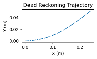
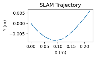
Trajctories from sitting the device on a desk
Notice that the SLAM plot shows far less movement than the dead reckoning plot, indicating that the WiFi SLAM algorithm is actually reducing the error of the raw IMU data.
To this end, we accomplished everything we said we would accomplish in our proposal.
In cases where the device is moved, our dead reckoning and SLAM plots are quite inaccurate, showing we moved tens of meters when we only moved two or three, and showing we moved in angles or made maneuvers that were definitely not executed in the test. Refer to the End-to-End testing section for examples.
Concusion
Given all of the testing and examples we have provided, we can conclude that we have completed a rough implementation of a WiFi SLAM system. Furthermore we did successfully create an embedded system capable of sampling data, preforming SLAM, and presenting results. As mentioned earlier, the algorithm we implemented is very sensitive to input movement data, and the naive dead reckoning approach does not give good distance measurements for this version of WiFi SLAM. Thus, below we outline some ideas for future work on this project.
Future Work
- Improve Dead Reckoning: The distance measurements were the achilles heel of this project, and improved dead reckoning would improve those. The first step would be to simply apply better filtering and gravity removal to the data. We could then look at more advanced dead reckoning approaches like the kalman filter.
- Try different sensor packages: For better WiFi measurement, we could use a discrete WiFi dongle that has a much better antenna and dynamic range. For movement, we could try using a wheel encoder to measure distance or velocity. This may be a much less error-prone method of collecting movement data rather than integrating acceleration twice to get distance.
- SLAM Performance Improvements: As discussed in the SLAM implementation section there is room for performance improvements in the SLAM algorithm. As it stands we can not collect large enough datasets to get results comparable to the paper because datasets that size would simply take too long to process.
- Use Acceleration data directly in SLAM: This is alternative to the improved dead reckoning strategy. We could import acceleration measurements directly into the SLAM algorithm and handle them in a similar fashion to the gyroscope measurements. This would not remove the need for better acceleration data filtering, but it would allow the algorithm to better correct for error in the data during the linearization step. It would also make the whole algorithm more theoretically sound as we would not be essentially performing half of dead reckoning before loading the data into SLAM.
- Try a different SLAM implementation: Graph SLAM is not the only game in town, and graph SLAM does not need to be implemented the way it was in this paper. Using the WiFi measurement function with different SLAM algorithms may lead to better results, or simpler SLAM algorithms.
- Try to not consolidate data before inputting it to SLAM: We now believe that associating each WiFi scan with one distance and angle was possibly not necessary. We would have liked to try not doing this and seeing if it improved the results. A potential issue with this approach is it would greatly increase the number of state variables, and thus the size of the matrices, further reducing our performance.
- Try testing in larger environments: The paper authors test in much larger environments than what we tested in, and they got plots accurate within 2 meters. Thus, if we only tested in 4 square meters of space, our error could be 50-100%. Thus, we would be curious what the results would be in a much larger environment, like a university building or school hallway.
Work Distribution

Willam Laney
wel53@cornell.edu
Implemented the WiFi SLAM code, unit tests, dead reckoning, and IMU data collection.

Luke Puchalla
lcp77@cornell.edu
Implemented WiFi data collection, and aided with TFT plotting and system integration.
Parts List
- Raspberry Pi 3B - Provided in lab
- PiTFT 2.8" Resistive Touchscreen - Provided in lab
- Wires and Breadboard - Provided in lab
- Sparkfun LSM9DS1 9DoF IMU Breakout - $16
- Optional: Your favorite USB WiFi dongle
Total: $16
References
WiFi SLAM
Efficient, Generalized Indoor WiFi GraphSLAMWiFi-SLAM Using Gaussian Process Latent Variable Models
Method of Improving WiFi SLAM based on Spatial and Temporal Coherence
Opportunistic Radio SLAM for Indoor Navigation using Smartphone Sensors
Utilizing WiFi signals for improving SLAM and person localization
Probabilistic Robotics
Datasheets
LSM9DS1 DatasheetPiTFT Datasheet
Software Documentation
NumPymatplotlib
Circuit Python
LSM9DS1 Circuit Python Library
Unittest
time
re
Code Appendix
All code can be found on GitHub
Notes
[1] Of course at other points, it makes the math much much harder ↩
[2] For a non-traditional SLAM solving technique that uses intense math instead of a measurement model see WiFi-SLAM Using Gaussian Process Latent Variable Models ↩
[3] https://youtu.be/mhVbLJvYP8s?t=49 ↩
[4] Accelerometers can not directly read the acceration due to gravity. However if the accelerometer is not in free fall it will read an acceration from the normal force resisting gravity. This is a subtle and confusing point, but it is important to understand for sucess working with accelerometers↩